
Take home additional 15 minute data for your plot selection by answering 5 short questions to help us do even better !
The Load Shape Library (LSL)TM and the Library PLUS 1.0 versions are intended to demonstrate basic features of Load Shape Profiling. The Load Shape Library is planned to evolve into a comprehensive tool with enhanced features and capabilities to house future end use load data collection activities by EPRI, electric utilities and other partners.
EPRI would like to thank the following entities for their support and contributions to the Load Shape Library.
The data is of value for improved end use load research for the benefit of load forecasters, system planners, energy efficiency program managers and rate design analysts for a variety of use cases.
About Customer Technologies Research at EPRI
About the Customer Technologies Website
Developed by/for:
Electric Power Research Institute (EPRI)
3420 Hillview Ave.
Palo Alto, CA 94304
Support for this Program is available from
EPRI Customer Assistance Center
Phone: 800-313-3774
Email:
askepri@epri.com
Copyright © 2012-2026 Electric Power Research Institute, Inc.
EPRI reserves all rights in the Program as delivered. The Program or any portion
thereof may not be reproduced in any form whatsoever except as provided by license
without the written consent of EPRI. A license under EPRI's rights in the Program
may be available directly from EPRI.
The embodiments of this Program and supporting materials may be ordered from
Electric Power Software Center (EPSC)
9625 Research Drive
Charlotte, NC 28262
Phone 1-800-313-3774
Email:
askepri@epri.com
For more information about EPRI and our extensive research portfolio, visit www.epri.com
THIS NOTICE MAY NOT BE REMOVED FROM THE PROGRAM BY ANY USER THEREOF.
NEITHER EPRI, ANY MEMBER OF EPRI, NOR ANY PERSON OR ORGANIZATION ACTING ON BEHALF
OF THEM:
1. MAKES ANY WARRANTY OR REPRESENTATION WHATSOEVER, EXPRESS OR IMPLIED, INCLUDING
ANY WARRANTY OF MERCHANTABILITY OR FITNESS OF ANY PURPOSE WITH RESPECT TO THE PROGRAM;
OR
2. ASSUMES ANY LIABILITY WHATSOEVER WITH RESPECT TO ANY USE OF THE PROGRAM OR ANY
PORTION THEREOF OR WITH RESPECT TO ANY DAMAGES WHICH MAY RESULT FROM SUCH USE.
RESTRICTED RIGHTS LEGEND: USE, DUPLICATION, OR DISCLOSURE BY THE UNITED STATES FEDERAL GOVERNMENT IS SUBJECT TO RESTRICTION AS SET FORTH IN PARAGRAPH (g) (3) (i), WITH THE EXCEPTION OF PARAGRAPH (g) (3) (i) (b) (5), OF THE RIGHTS IN TECHNICAL DATA AND COMPUTER SOFTWARE CLAUSE IN FAR 52.227-14, ALTERNATE III.
Open All
Close All
-
+
-
+
-
+
-
+
Introduction
The regulated U.S. utility industry relies on customer load shapes and class load profile data for the recovery of their fixed costs estimated at USD 165 billion in 2010. Understanding class load shapes requires end-use data for gaining insights into drivers, uncertainties and behaviors of customer loads. End-Use load data currently available to the industry was developed 20 years ago by a few utilities and EPRI. End-Use energy consumption patterns have changed significantly over the years due to efficient technologies, new loads, new building codes, customer behaviors and preferences for the use of electricity. This fundamental change has created a challenge to the industry for acquiring and compiling recent and representative load data. How can utilities acquire or gain access to recent load data through EPRI’s research or through other collaborative efforts? How can Utilities deploy EPRI’s analytical framework to develop their own representative end-use and whole premise load data libraries by attributes such as region, climate zone, sector and building type?
Utilities continue to express the need for more recent end use and whole premise data. Such data is generally believed to be prohibitively expensive to acquire and process. The wide-spread deployment of AMI (Advanced metering infrastructure) meters creates both opportunities and challenges for collection, management and storage of large volumes of data. The opportunity that AMI meters present is that whole-premise load shapes can be measured without the need for special additional metering. The challenge is that the quantities of data being collected are very large (terabytes) needing enormous data storage resources and investment decisions for establishing processing and rigorous sampling structures. Additional resource and cost challenges exist for retention of adequate amounts of data for extended periods of time.
AMI meters installed at the premise, however, will not provide end-use level load shapes, which can be very important to understanding how new technologies impact the overall load shape over time, as well as how customers respond to dynamic pricing, information feedback, and demand response program options. Limited research has been conducted till date to determine whether low cost techniques such as statistical estimation of end use load consumption using survey information and whole premise load data, yield accurate estimates. More research is needed to determine the accuracy of these lower-cost techniques or whether collaborative approaches to funding alternative end-use load research measurement methods would be the desirable next step.
Rationale
In a 2010 EPRI survey, utilities and ISOs mentioned the increasing need for acquiring high-quality load research data. Utility representatives mentioned that the utility industry as a whole are using “antique” load shape data for forecasting, planning, and program design purposes—load shapes that the industry and EPRI developed more than 20 years ago. The industry is concerned about the accuracy of load forecasts as the forecasts are based on these “antique” load shapes.1
In May 2012, EPRI conducted a workshop for utilities and non-utility stake holders interested in load research and in collecting load data. Participants reiterated the need for more recent load data to improve load forecasting accuracy, energy efficiency program design and for integrating energy efficiency and demand response into resource planning. There was unanimous consensus for the creation of a framework for the development of a load shape library or repository for storing, processing and navigating end-use and whole-premise load data.
Objectives
The objectives of the load shape library effort are as follows:
- Develop a preliminary framework (database and a secure web portal) with best-available end use, whole premise, technology measures and pacific northwest rbsa load data by region, climate zone, sector and building type to demonstrate the design and basic functionality of the repository.
- Continue to revise the framework annually and populate the library with newer end use and whole premise data as available from EPRI research and/or from external agencies such as utilities and others.
Applications, Value and Use
End-use and whole-premise load shapes find utility applications in load forecasting, integrated resource planning (IRP) and demand-side management (DSM) evaluations. Some utilities are required to submit predicted load growth and future capacity needs to the public utility commission (PUC), considering factors such as the current base load, expected change in the number of residential, commercial and industrial establishments and change in equipment efficiencies over time. Base load energy, coincident peak and impact of equipment efficiencies can be quantified by sector and over specific durations of time using end-use and whole-premise load shapes. When DSM programs are selected and implemented it is because they have been determined to be cost effective based on assumed energy and/or demand savings and program administrative costs. In order to improve these assumptions, several PUCs require that evaluations be performed to determine the true savings and the program costs, respectively known as impact evaluation and process evaluation. Impact evaluations can be performed using one of many approaches namely end-use metered data, whole premise load research data, billing history analysis, building simulation and other statistical methods. Such approaches can use end-use load shapes and/or whole-premise load data to capture the change in energy use patterns resulting from DSM programs.
References
1. End-Use Load Research in a Smart Grid World: Conference Proceedings. EPRI, Palo Alto, CA: 2010. 1020122↩
This section describes the load shape library developed during the year . The library comprises of the following four component databases containing hourly and fifteen-minute load data, accessible from the download options on the portal.
Open All
Close All
-
+
How was the end-use load data derived?
The end-use load shape data contained in the tool is derived from simulations using the EPRI NESSIE (National Electric System Simulation Integrated Evaluator) model platform. The inputs to NESSIE are derived from data estimated by the U.S. Energy Information Agency’s (EIA) National Energy Modeling System (NEMS) as well as from data collected by EPRI through its laboratory testing and research. 1
-
+
How is the data displayed in the end-use load shape library?
The end use load data available in the tool are average hourly demand values unitized to the respective end-use peak. The unitized end use peak value is the maximum value of 1.0 for the season (peak/off-peak) and for the day type (peak day, average weekday, and average weekend) selected by the user. The tool allows scaling the unitized end use load data based on the user’s input of peak end use kW or annual end use kWh.
-
+
What regions are represented in the end-use load shape data?
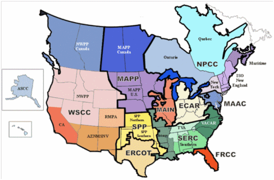
The EPRI NESSIE model simulated unitized hourly demand values for thirteen (13) North American Electric Reliability Corporation (NERC) regions and sub-regions according to the NERC pre-2006 regional designations excluding Alaska and Hawaii. Figure 2-1 illustrates the geographic distinctions of the thirteen NERC regions for which data is available in the end-use load shape library. Table 2-1 enlists the names of the thirteen NERC regions and sub-regions and the abbreviations used.
Figure 2-1
Geographic Depiction of Pre-2006 NERC Control Regions
Geographic Depiction of Pre-2006 NERC Control Regions
| NERC Region/Subregion | Abbreviation |
|---|---|
| East Central Reliability Coordination Agreement | ECAR |
| Electric Reliability Council of Texas | ERCOT |
| Mid-Atlantic Area Council | MAAC |
| Mid-America Interconnected Network | MAIN |
| Mid-Continent Area Power Pool | MAPP |
| Northeast Power Coordinating Council – New York | NPCC/NY |
| Northeast Power Coordinating Council – New England | NPCC/NE |
| Southeast Reliability Council (non-Florida) | SERC/STV |
| Southeast Reliability Council (Florida) | SERC/FL |
| Southwest Power Pool | SPP |
| Western States Coordinating Council – Northwest | WSCC/NWP |
| Western States Coordinating Council – Rocky Mountain Area | WSCC/RA |
| Western States Coordinating Council – California/Nevada | WSCC/CNV |
Table 2-1
Pre-2006 NERC Regions and Subregions represented in the End-use Load Shape Data
Pre-2006 NERC Regions and Subregions represented in the End-use Load Shape Data
-
+
How are the sectors and end-uses defined?
Unitized hourly demand values available in the database pertain to end-uses of three sectors namely residential, commercial, and industrial corresponding to each of the 13 NERC regions and sub-regions described above. To generate the end use load data in each case, regional prototypes were used to represent different building or business types. Auxiliary data sources were used to find the saturation of the selected building or business types by state and mapping back to the appropriate NERC region. The frequency counts of saturation were then used as weights to calculate a weighted average load shape for each end-use for the specific NERC region. A total of twenty-two (22) major end use load categories across residential, commercial, and industrial sectors for each NERC region and sub-region were developed as shown in Table 2-2.
| Residential End-uses (9) | |
|---|---|
| Central Air Conditioning (CAC) | Heating |
| Clothes Dryer | Lighting |
| Clothes Washer | Refrigerator |
| Dishwasher | Television and Personal Computer (TV & PC) |
| Water Heating | Commercial End-uses (8) |
| Cooling | Office Equipment |
| Heating | Refrigeration |
| Lighting, External | Ventilation |
| Lighting, Internal | Water Heating | Industrial End-uses (5) |
| HVAC | Machine Drives |
| Lighting | Process Heating |
| Other |
Table 2-2
Twenty-two (22) End-uses Included in the Load Shape Library
Twenty-two (22) End-uses Included in the Load Shape Library
-
+
How are the season and day-types defined?
The load shapes were condensed into two season types and four day types each consisting of twelve (12) two-hour blocks of energy use. Extrapolations were used to convert the values into twenty-four (24) hour format. The season and day type definitions are as follows:
- Peak season: Months of May through September.
- Off-peak season: Months of October through April.
- Peak weekday in the peak season: Ten hottest weekdays that are not holidays two in each of the months for the peak season namely May through September.
- Peak weekday in the off-peak season: Ten coldest (or hottest weekdays depending on region) that are not holidays, for the months of the off-peak season namely October through April.
- Average weekday/weekend in the peak season: all other weekdays/weekends in May through September.
- Average weekday/weekend in the off-peak season: all other weekdays/weekends in October through April.2
Open All
Close All
-
+
What can I expect to find in the whole-premise load shape library?
The whole-premise load shape data is obtained from the PowerShape™ database of load shapes developed by EPRI's Center for End-Use Energy Data (CEED). 2 The data was produced using statistical models using step-wise linear regression techniques, metered end-use data, and the corresponding historic weather data. Typically 5 to 15 validated (pre-screened for proper characteristics and data quality) sites are utilized to construct the shape. For instance in the regression process, the relationship between the donor sites’ metered hourly HVAC energy consumption (using hourly metered end-use data) and the corresponding metered hourly temperature-humidity index (a function of dry bulb temperature and dew point) is statistically quantified.
Salient features of the CEED data is listed below:
- Data is presented as “total load” or “whole-premise” energy load shapes for various commercial and residential sector building types.
- Load shapes are diversified i.e. the shape represents a group of customers in a particular sector and not an individual customer.
- The load shapes are for the calendar year 2001 and make use of “normal”3 and Typical Meteorological Year (TMY2)4 weather data.
- The load shapes can be described as typical, weather-adjusted, load profiles for selected sectors, by state and city.
- The diversified load shapes are accompanied by attributes and tools that enable analysis to be conducted at both the individual customer and sector levels.
-
+
How is the whole-premise data presented to the user?
The whole premise load shape data is presented 8760 format i.e. one energy value (kWh for residential and Wh per square foot for commercial) for each hour of the calendar year 2001.
-
+
What sectors and building types are represented?
The data consists of load shape data for residential and commercial sectors. Weather-adjusted data for nine (9) residential premise types (Table 2-3) and thirty (30) commercial building types ( Table 2-4 ) for fifty-five (55) U.S. cities is included. The weather adjustments are based on hourly “normal” weather data for most cities and Typical Meteorological Year (TMY2) data for the others. The premise types are classified according to the use of electric and fossil fuel for heating. Therefore, a combined total of 4173 class load segment profiles are available for users in this tool.
| Residential Premise Type | Description |
|---|---|
| Single Family, Heat Pump AC | Heat Pump Heating and Cooling |
| Single Family, Central AC | Electric Heating (non-Heat Pump) with Central Air |
| Single Family, Large | Large All-electric Customer (large home, 2 or more children) |
| Single Family, Mixed Cooling | Fossil Heat with Mixed Cooling |
| Single Family, Central AC, Elec.WH | Fossil Heat with Central Air and with Electric Water Heater |
| Multi-Family, Mixed Cooling | Electric Heating and Mixed Cooling |
| Multi-Family, Room AC | Fossil Heating with Room Air |
| Manufactured Home, Mixed Cooling | Electric Heat and Mixed Cooling |
| Manufactured Home, Mixed Cooling | Fossil Heat and Mixed Cooling |
Table 2-3
Nine (9) Weather-Adjusted Residential Premise Types
Nine (9) Weather-Adjusted Residential Premise Types
| Commercial Building Type | Description |
|---|---|
| Office | Small Offices - Electric Heat |
| Office | Medium Offices -Electric Heat |
| Office | Large Offices - Electric Heat |
| Office | Small Offices - Fossil Heat |
| Office | Medium Offices - Fossil Heat |
| Office | Large Offices - Fossil Heat |
| Education | Schools (K-12) - Electric Heat |
| Education | Schools (K-12) - Fossil Heat |
| Restaurant | Fast Food Restaurant – Typical |
| Restaurant | Fast Food Restaurant – Burgers & Breakfast |
| Restaurant | Sit-down Restaurant |
| Healthcare | Mixed Usage Healthcare - Hospitals & Nursing Homes |
| Retail | Small Retail - Electric Heat |
| Retail | Large Retail - Electric Heat |
| Retail | Small Retail - Fossil Heat |
| Retail | Large Retail - Fossil Heat |
| Lodging | Hotels/Motels - Electric Heat |
| Lodging | Hotels/Motels - Fossil Heat |
| Assembly | Churches – Electric Heat |
| Assembly | Churches - Fossil Heat |
| Entertainment | Movie Theaters – Fossil Heat |
| Warehouse | Warehouse – Fossil Heat |
| Services – Other | Banks – Financial Services – Electric Heat |
| Services – Other | Banks – Financial Services – Fossil Heat |
| Grocery | Supermarkets |
| Grocery | Convenience Stores: 24-hour Operation |
| Grocery | Convenience Stores: non 24-hour Op. |
| Retail | Malls – Fossil Heat |
| Transport-Public Utilities | Trucking - Distribution Center |
| Transport-Public Utilities | Communication Facilities – General |
Table 2-4
Thirty (30) Weather-Adjusted Commercial Building Types
Thirty (30) Weather-Adjusted Commercial Building Types
-
+
What cities and states are represented?
The tables below show the cities and respective states for which whole-premise load shapes are available. The cities and states are grouped by geographic region along with annual HDD (heating degree day) and annual CDD (cooling degree day) counts.
Midwest
A group of ten (10) cities from the Midwest region are included in the database (Table 2-5). These include two (2) cities from Illinois, (7) seven from Ohio and (1) one from Michigan.
| Region | State | City | Weather Station | Annual HDD | Annual CDD |
|---|---|---|---|---|---|
| Midwest | IL | CHICAGO | 94846 | 6481 | 778 |
| Midwest | IL | SPRINGFIELD | 93822 | 5846 | 1166 |
| Midwest | MI | LANSING | 14836 | 7110 | 552 |
| Midwest | OH | AKRON | 14895 | 6176 | 641 |
| Midwest | OH | CLEVELAND | 14820 | 6132 | 655 |
| Midwest | OH | COLUMBUS | 14821 | 5576 | 837 |
| Midwest | OH | DAYTON | 93815 | 5818 | 818 |
| Midwest | OH | MANSFIELD | 14891 | 6248 | 686 |
| Midwest | OH | TOLEDO | 94830 | 6646 | 649 |
| Midwest | OH | YOUNGSTOWN | 14852 | 6506 | 541 |
Table 2-5
Midwest Cities Included in the Whole-premise Database
Midwest Cities Included in the Whole-premise Database
Northeast
A group of eleven (11) cities from the Northeast region are included in the database (Table 2-6). These include four (4) cities from Pennsylvania, two (2) cities each from New York and New Jersey and (1) one city each from Massachusetts, New Hampshire and Vermont.
| Region | State | City | Weather Station | Annual HDD | Annual CDD |
|---|---|---|---|---|---|
| Northeast | MA | BOSTON | 14739 | 5768 | 699 |
| Northeast | NH | CONCORD | 14745 | 7601 | 416 |
| Northeast | NJ | ATLANTIC CITY | 93730 | 5221 | 908 |
| Northeast | NJ | NEWARK | 14734 | 4994 | 1138 |
| Northeast | NY | ALBANY | 14735 | 7003 | 539 |
| Northeast | NY | ROCHESTER | 14768 | 6734 | 596 |
| Northeast | PA | HARRISBURG | 14751 | 5469 | 1017 |
| Northeast | PA | PHILADELPHIA | 13739 | 5005 | 1133 |
| Northeast | PA | PITTSBURGH | 94823 | 5932 | 700 |
| Northeast | PA | WILKES-BARRE | 14777 | 6494 | 575 |
| Northeast | VT | BURLINGTON | 14742 | 7843 | 438 |
Table 2-6
Northeast Cities Included in the Whole-Premise Database
Northeast Cities Included in the Whole-Premise Database
South
A group of twenty-two (22) cities from the southern region are included in the database (Table 2-7). These include seventeen (17) cities from Texas two (2) cities from North Carolina and one (1) city each from Florida, Georgia, and Maryland.
| Region | State | City | Weather Station | Annual HDD | Annual CDD |
|---|---|---|---|---|---|
| South | FL | MIAMI | 12839 | 145 | 4206 |
| South | GA | ATLANTA | 13874 | 2982 | 1690 |
| South | MD | BALTIMORE | 93721 | 4790 | 1177 |
| South | NC | CHARLOTTE | 13881 | 3344 | 1560 |
| South | NC | GREENSBORO | 13723 | 3965 | 1282 |
| South | TX | ABILENE | 13962 | 2621 | 2325 |
| South | TX | AMARILLO | 23047 | 4475 | 1328 |
| South | TX | AUSTIN | 13958 | 1644 | 2927 |
| South | TX | BROWNSVILLE | 12919 | 626 | 3720 |
| South | TX | CORPUS CHRISTI | 12924 | 907 | 3349 |
| South | TX | EL PASO | 23044 | 2594 | 2091 |
| South | TX | FORT WORTH | 3927 | 2356 | 2523 |
| South | TX | HOUSTON | 12960 | 1540 | 2827 |
| South | TX | LUBBOCK | 23042 | 3430 | 1641 |
| South | TX | LUFKIN | 93987 | 1903 | 2517 |
| South | TX | MIDLAND | 23023 | 2732 | 2051 |
| South | TX | PORT ARTHUR | 12917 | 1496 | 2754 |
| South | TX | SAN ANGELO | 23034 | 2351 | 2388 |
| South | TX | SAN ANTONIO | 12921 | 1627 | 2929 |
| South | TX | VICTORIA | 12912 | 1182 | 3066 |
| South | TX | WACO | 13959 | 2118 | 2679 |
| South | TX | WICHITA FALLS | 13966 | 3040 | 2371 |
Table 2-7
Southern Cities Included in the Whole-premise Database
Southern Cities Included in the Whole-premise Database
West
Finally, twelve (12) cities from the western region are included in the database (Table 2-8). These include three (3) cities from Arizona, six (6) cities from California and one (1) city each from Montana, Nevada, and Oregon.
| Region | State | City | Weather Station | Annual HDD | Annual CDD |
|---|---|---|---|---|---|
| West | AZ | FLAGSTAFF | 3103 | 7208 | 115 |
| West | AZ | PHOENIX | 23183 | 1099 | 4020 |
| West | AZ | TUCSON | 23160 | 1540 | 2852 |
| West | CA | FRESNO | 93193 | 2510 | 1924 |
| West | CA | LOS ANGELES | 23174 | 1268 | 559 |
| West | CA | SACRAMENTO | 23232 | 2641 | 1211 |
| West | CA | SAN DIEGO | 23188 | 1050 | 803 |
| West | CA | SAN FRANCISCO | 23234 | 3046 | 97 |
| West | CA | SANTA MARIA | 23273 | 2957 | 76 |
| West | MT | HELENA | 24144 | 7899 | 301 |
| West | NV | LAS VEGAS | 23169 | 2273 | 3087 |
| West | OR | MEDFORD | 24225 | 4674 | 689 |
Table 2-8
Western States Included in the Whole-Premise Database
Western States Included in the Whole-Premise Database
-
+
How are the season and day-types defined?
The load shapes were condensed into two season types and four day types each consisting of twelve (12) two-hour blocks of energy use. Extrapolations were used to convert the values into twenty-four (24) hour format. The season and day type definitions are as follows:
- Peak season: Months of May through September.
- Off-peak season: Months of October through April.
- Peak weekday in the peak season: Ten hottest weekdays that are not holidays two in each of the months for the peak season namely May through September.
- Peak weekday in the off-peak season: Ten coldest (or hottest weekdays depending on region) that are not holidays, for the months of the off-peak season namely October through April.
- Average weekday/weekend in the peak season: all other weekdays/weekends in May through September.
- Average weekday/weekend in the off-peak season: all other weekdays/weekends in October through April.1
References
1. Modeling CO2 Emissions Impact of Energy Efficiency: Proof of Concept. EPRI, Palo Alto, CA:2008. 1016085↩
2. PowerShape Market Profiles, EPRICSG, Palo Alto, CA: 1999. TR-111998↩
3. U.S. National Oceanic and Atmospheric Administration (NOAA) 1981-2010 Climate Normal Data https://www.ncdc.noaa.gov/cdo-web/datatools/normals ↩
4. For definition of TMY2 weather data format see http://rredc.nrel.gov/solar/pubs/tmy2/pdfs/tmy2man.pdf ↩
Open All
Close All
-
+
Where can I find information about the Technology Measures load shape library?
The technology measures load data is obtained from EPRI's Energy Efficiency Technology Demonstration 1.0 project conducted during 2009-2013. The data pertains to field installed residential efficient end-use technologies namely Heat Pump Water Heaters (HPWH) and Efficient Appliances (Washers, Dryers and Refrigerators) deployed with extensive measurement instrumentation at multiple sites throughout the United States.
The objectives of the Energy Efficient Technology Demonstration were as follows:
- Examine the efficiency and performance of the technologies.
- Assess energy savings for different climatic regions and different building designs and constructions.
- Identify and quantify different qualities and effects when compared with traditional technology.
- Identify changes necessay in building designs and construction to attain optimal levels of energy performance and savings.
- Understand technical obstacles such as the possible impact that the technologies may have on the performance of the electric grid.
- Examine the feasibility of applying efficiency standards.
EPRI designed the overall scope and managed the demonstrations project hosted by multipled utilities. Within the scope of the project, EPRI identified and qualified the technologies for demonstration, worked with manufacturers to secure their availability, created the demonstration protocol, ran and executed tests, and performed an evaluation of the preliminary data.
Load data for two technology measures as described below is available in the current version of Load Shape Library. The data also consists of conventional or base technology data for each of the technology measures1.
-
+
How do heat pump water heaters work and how are
they represented in the Technology Measures load shape library?
HPWHs use electricity to move heat from the ambient to the water heater storage tank to heat water. During cold ambient conditions the Heat pump water heater operates like a conventional water heater to directly heat water. The main diversity factors affecting technical performance are climate region and location of the heat pump water heater within the residential site. Data for two differnt HPWM models anonymized as "Manufacturer A" and "Manufacturer B" is included in the database. Conventional water heaters included in the data include all manufacturers and brands available in customer sites during the period of the project.
-
+
What appliances are represented and what features help make them energy efficient?
Three residential standalone appliances namely refrigerators, washers and dryers are included. The efficient refrigerators use innovative technology, such as inverter-driven compressors and automatic ice-makers. The efficient washers are front-loaded designs and other features that reduce water consumption and electricty use. The efficient dryers use electronically controlled brushless motors and efficient air flow designs to reduce electric consumption. The key diversity factor for residential appliance performance is the usage of the device (how often and how long) which is driven by demographic characteristics such as number of occupants and the age of occupants.
Open All
Close All
-
+
What makes up the Pacific Northwest RBSA load shape library?
The RBSA is a study sponsored by the Northwest Energy Efficiency Alliance (NEEA) in the Pacific Northwest region. The primary objective of the RBSA was to develop an inventory and profile of existing residential building stock in the Northwest based on field data from a representative, random sample of existing homes. The RBSA establishes the 2011 regional baseline for housing stock for three categories of residences: single-family homes, manufactured homes, and multifamily homes. The dataset used in the Load Shape Library comprises of the following:
- 103 single-family residential premises with end-use metered data
- The data ranges from April 2012- April 2013
- Data includes premises with electric and gas end-uses
EPRI used the dataset and the data contained within RBSA public database. No changes, or modifications or validations were conducted on the data except for the exclusion of gas end uses 1.
-
+
How was the data collected?
Three different data collection methods were applied, each depended on the end-use being measured.
- Direct whole-premise and major loads were measured directly at the electrical panel
- Appliances and electronics were measured using plug measurement nodes
- Lighting fixtures were measured using stand-alone data loggers
-
+
What format is the data available in?
The Pacific Northwest RBSA load data available in the tool are average hourly and daily demand values presented in 8760 format i.e. one energy value (kWh) and day type (average weekday, average weekend and average weekdays and weekends). Extrapolations were used to convert the values into hourly and daily formats.
-
+
What cities and States are represented in the Pacific Northwest RBSA load shape library?
The NEEA metered data consists of load shape data for single family residential homes in three sampling regions: Puget Sound, western Oregon and the eastern region composed of eastern Washington, Idaho and western Montana. The group of tables below enlists the cities represented in each state.
Idaho
Thirteen (13) cities from Idaho are included in the database (Table 2-9).
| City | State |
|---|---|
| Boise | ID |
| Caldwell | ID |
| Coeur d Alene | ID |
| Emmett | ID |
| Jerome | ID |
| Kuna | ID |
| Lewiston | ID |
| Meridian | ID |
| Moscow | ID |
| Mountain Home | ID |
| Nampa | ID |
| Sandpoint | ID |
| Shoshone | ID |
Table 2-9
Idaho cities included in the Pacific Northwest RBSA database
Idaho cities included in the Pacific Northwest RBSA database
Montana
Five (5) cities from Montana are included in the database (Table 2-10).
| City | State |
|---|---|
| Bozeman | MT |
| Cascade | MT |
| Hamilton | MT |
| Helena | MT |
| Whitehall | MT |
Table 2-10
Montana cities included in the Pacific Northwest RBSA database
Montana cities included in the Pacific Northwest RBSA database
Oregon
Sixteen (16) cities from Oregon are included in the database (Table 2-11).
| City | State |
|---|---|
| Albany | OR |
| Bandon | OR |
| Beaverton | OR |
| Brookings | OR |
| Carlton | OR |
| Dundee | OR |
| Eugene | OR |
| Hillsboro | OR |
| Jefferson | OR |
| Lake Oswego | OR |
| Lebanon | OR |
| McMinnville | OR |
| Monmouth | OR |
| Portland | OR |
| Salem | OR |
| South Beach | OR |
Table 2-11
Oregon cities included in the Pacific Northwest RBSA database
Oregon cities included in the Pacific Northwest RBSA database
Washington
Thirty-two (32) cities from Washington are included in the database (Table 2-12).
| City | State |
|---|---|
| Airway Heights | WA |
| Arlington | WA |
| Bainbridge Island | WA |
| Bellevue | WA |
| Bellingham | WA |
| Bothell | WA |
| Burien | WA |
| Cheney | WA |
| East Wenatchee | WA |
| Fox Island | WA |
| Grandview | WA |
| Kennewick | WA |
| Kettle Falls | WA |
| Kirkland | WA |
| Lynnwood | WA |
| Mill Creek | WA |
| Moses Lake | WA |
| Mountlake Terrace | WA |
| Newport | WA |
| Oak Harbor | WA |
| Okanogan | WA |
| Olympia | WA |
| Puyallup | WA |
| Renton | WA |
| Seattle | WA |
| Spokane | WA |
| Spokane Valley | WA |
| Tacoma | WA |
| Tenino | WA |
| Wenatchee | WA |
| West Richland | WA |
| Yakima | WA |
Table 2-12
Washington cities included in the Pacific Northwest RBSA database
Washington cities included in the Pacific Northwest RBSA database
-
+
How many utilities are represented in each state?
Twenty-nine (29) utilities across the four states are represented in the database. This includes three (3) utilities in Idaho, three utilities (3) in Montana, eight (8) utilities in Oregon and seventeen (17) utilities in Washington (Table 2-13).
| Number of Utilities Per State | State |
|---|---|
| 3 | ID |
| 3 | MT |
| 8 | OR |
| 17 | WA |
Table 2-13
Number of utilities per state included in the Pacific Northwest RBSA database
Number of utilities per state included in the Pacific Northwest RBSA database
References
1. RBSA Single-Family Public Data Files https://neea.org/data/residential-building-stock-assessment ↩
This section details a sample set of instructions for using the Load Shape Library . The tool is self-explanatory in the selections and choices the user can opt.
Open All
Close All
-
+

How can I access the End-use and Whole-premise Load Shape libraries?
Steps to Access End Use and Whole Premise Load Shapes
Step 1:
Log into the web portal loadshape.epri.com from a web browser such as Internet Explorer version 8.0 or higher, Mozilla Firefox, or Google Chrome. The web portal also can be accessed using mobile devices such as Apple or Android based smartphones and tablets.
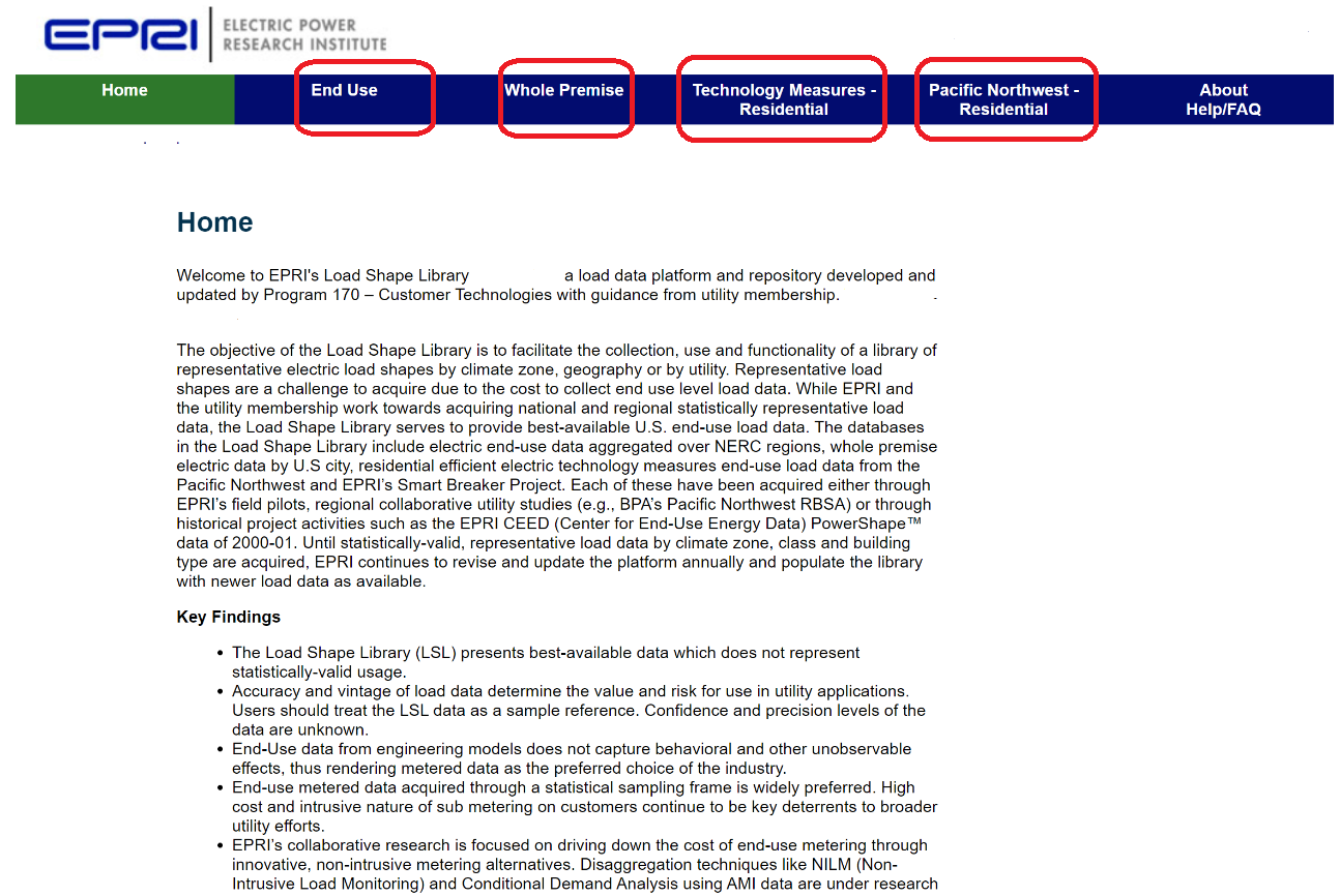
The user arrives at the home page of the Load Shape Library as shown in Figure 3-1.
Figure 3-1
Load Shape Library home page
Load Shape Library home page
Step 2:
From the home page the user can chose either to access the end use load shape library, the whole premise load shape library, the technology measures library or the Pacific Northwest RBSA library as shown in Figure 3-2 . The instructions below start with the assumption that the user chooses to access the end use load shape library first.
Step 3:
The user selects the end use load shape library from the database options on the home page as shown highlighted in red (Figure 3-2).
Figure 3-2
End Use and Whole Premise Database Options
End Use and Whole Premise Database Options
Step 4:
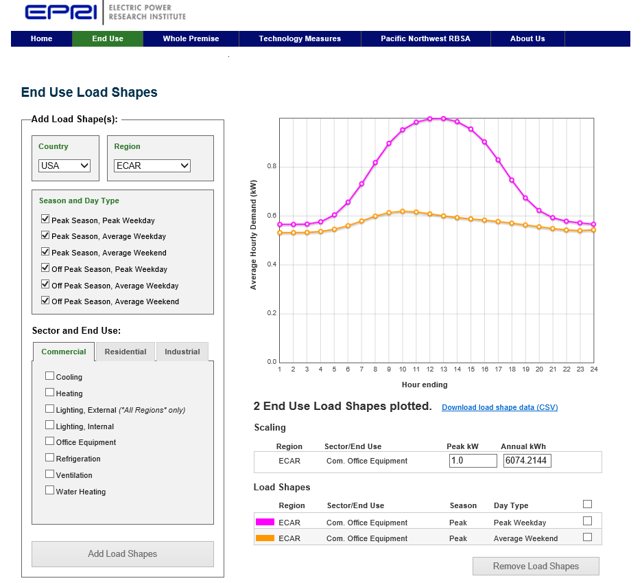
Figure 3-3 shows the end use load shape library page and the selections available for the user to access, visualize and download the desired end use data.
Figure 3-3
End Use Load Shape Library and Selection Options
End Use Load Shape Library and Selection Options
The user chooses the country and region for which load data is desired. The user then selects the desired season and day type, followed by the sector and end use of interest. The user may select any combination of region, season, and day type for a maximum of sixteen (16) end use load shapes. The user then clicks the "Add Load Shapes" button at the bottom left to display the unitized end use load shapes stacked one above the other as shown in Figure 3-3. The load shapes are displayed in different colors for contrast. The user can enter one of the scaling factors namely Peak kW or Annual kWh for the specific end use to obtain the desired load shape in kW values (y-axis) by hour (x-axis).
Below the plot is a displayed table which the user may use to remove one or more selections. The load shape plots can be removed by checking the appropriate checkbox(es) on the far right side of the label denoting the plot and clicking the "Remove Load Shapes" button.
A blue hyperlink ("Download load shape data(CSV)") is available below the chart. It allows the user to download the data displayed on the chart, along with the selection specifics such as region, sector, end use and day type associated with each plot.
Step 5:
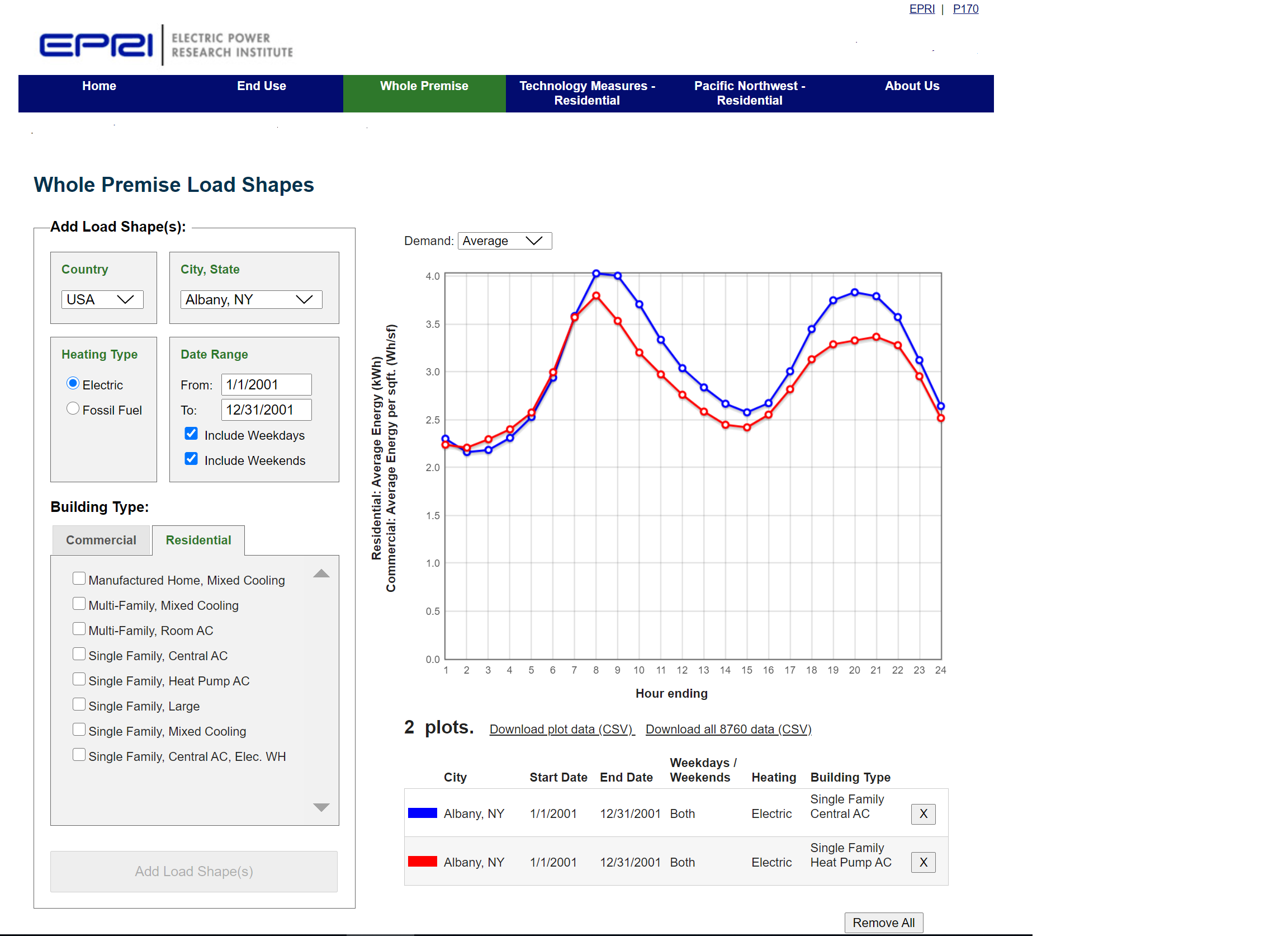
Figure 3-4 shows the whole premise load page and the selections available to the user for accessing whole premise load shape data. The menus and features available for the user are similar to the ones described above for the end use library. Additional filters to display load shapes for average day, week, month, year and single hour are provided. The default setting for demand values (displayed on the y-axis) is "average". For select menus the load shapes can be generated using maximum or minimum demand values.
Figure 3-4
Whole Premise Load Shape Library and Selection Options
Whole Premise Load Shape Library and Selection Options
Open All
Close All
-
+
How can I access the Technology Measures Load Shape library?
Steps to Access Technology Measure Load Shapes
Step 1:
Log into the web portal loadshape.epri.com from a web browser such as Internet Explorer version 8.0 or higher, Mozilla Firefox, or Google Chrome. The web portal also can be accessed using mobile devices such as Apple or Android based smartphones and tablets.
The user arrives at the home page of the Load Shape Library.
Step 2:
From the home page the user can chose either to access the end use load shape library , the whole premise load shape library, the technology measures library or the pacific northwest rbsa library. The instructions below start with the assumption that the user chooses to access the technology measures library first.
Step 3:
Figure 3-6 shows the User choosing one of the four geographic selections for which load shape data is desired. In the screenshot below, user selects “Mixed-Humid” and “Hot-Humid” Climate zones.
Figure 3-6
Technology Measures Geographic Selection
Technology Measures Geographic Selection
Step 4:
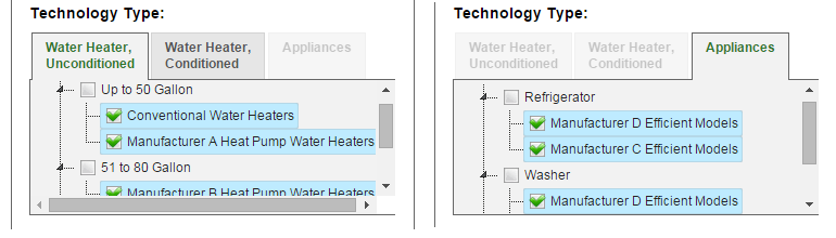
Figure 3-7 shows how the user can select a technology type namely Water Heaters or Appliances. For water heaters the user can select the units located in unconditioned spaces and/or in conditioned spaces. If available under the selected geography (City, Utility or Climate Zone) water heaters can be selected by tank size such as: up to 50 gallons, 51-80 gallons and exceeding 80 gallons. For each water heater size, user can select conventional (or electric resistance) and/or Heat Pump Water Heaters as available. Data concerning Heat Pump Water Heaters from different manufacturers such as A and B are available for user selection.
For Appliances the user can choose from Refrigerators, Washers and Dryers if available under the selected geography (City, Utility or Climate Zone). For each of the three appliances conventional and/or efficient units can be selected if data is available. Efficient units from different manufacturers such as A, B, C and D are available for user selection.
Figure 3-7
Technology Measures Technology Type Selection
Technology Measures Technology Type Selection
Step 5:
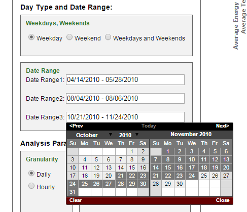
Figure 3-8 shows the selections for day type and date range. User can select load shapes computed for weekdays or weekends or both over the desired date range selected using the calendar option as shown. Three date ranges (1, 2, and 3) enable user to choose up to three discreet time blocks (days, weeks or months) if needed. This is useful in selecting system peak days and off peak days or three season blocks such as shoulder season 1, shoulder season 2 and peak season. User can also choose a combination of contiguous time blocks and discrete time blocks.
In the screenshot shown below, user selects weekday load shapes for three periods as 04/14/2010-05/28/2010, 08/04/2010-08/06/2010 and 10/21/2010-11/24/2010.
Figure 3-8
Technology Measures Season Type Selection
Technology Measures Season Type Selection
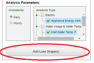
Step 6:
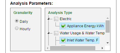
User selects the analysis parameters namely the granularity of the load data (hourly or daily) and the analysis type. The analysis type can be electric, water usage, temperature or other performance variable such as COP (coefficient of performance). It is important to note that the analysis type variable is an average quantity. For example, if user selects hourly granularity for Appliance Energy kWh, then the energy for the selected appliance is averaged on an hourly basis over the date range selected.
In the screenshot shown in Figure 3-9, user selects two parameters namely daily load data for Appliance energy kWh and the corresponding daily inlet water temperature in F.
Figure 3-9
Technology Measures Analysis Type Selection
Technology Measures Analysis Type Selection
Step 7:
User then hits the “Add Load Shape(s) button to display the load shapes.
Figure 3-10
Technology Measures Submit
Technology Measures Submit
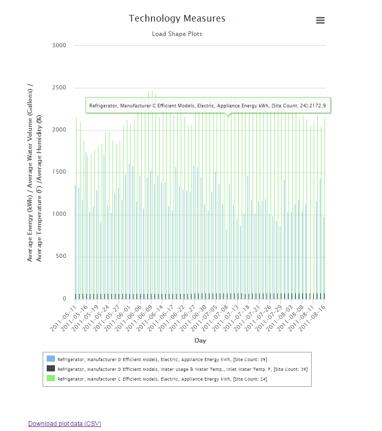
Step 8:
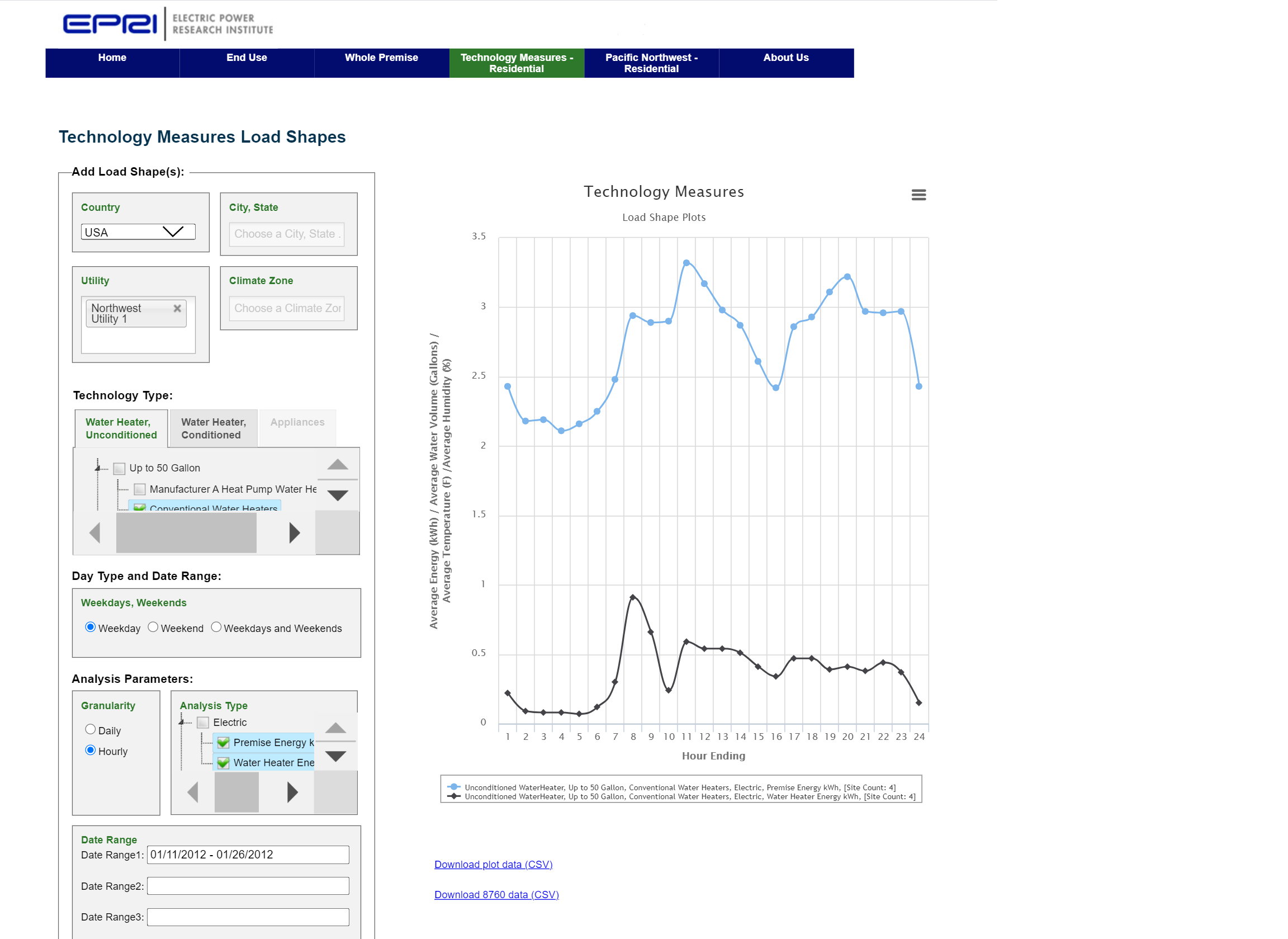
The Load Shape is displayed if data is available for the selections, the user made.
Figure 3-11
Technology Measures Data Plot
Technology Measures Data Plot
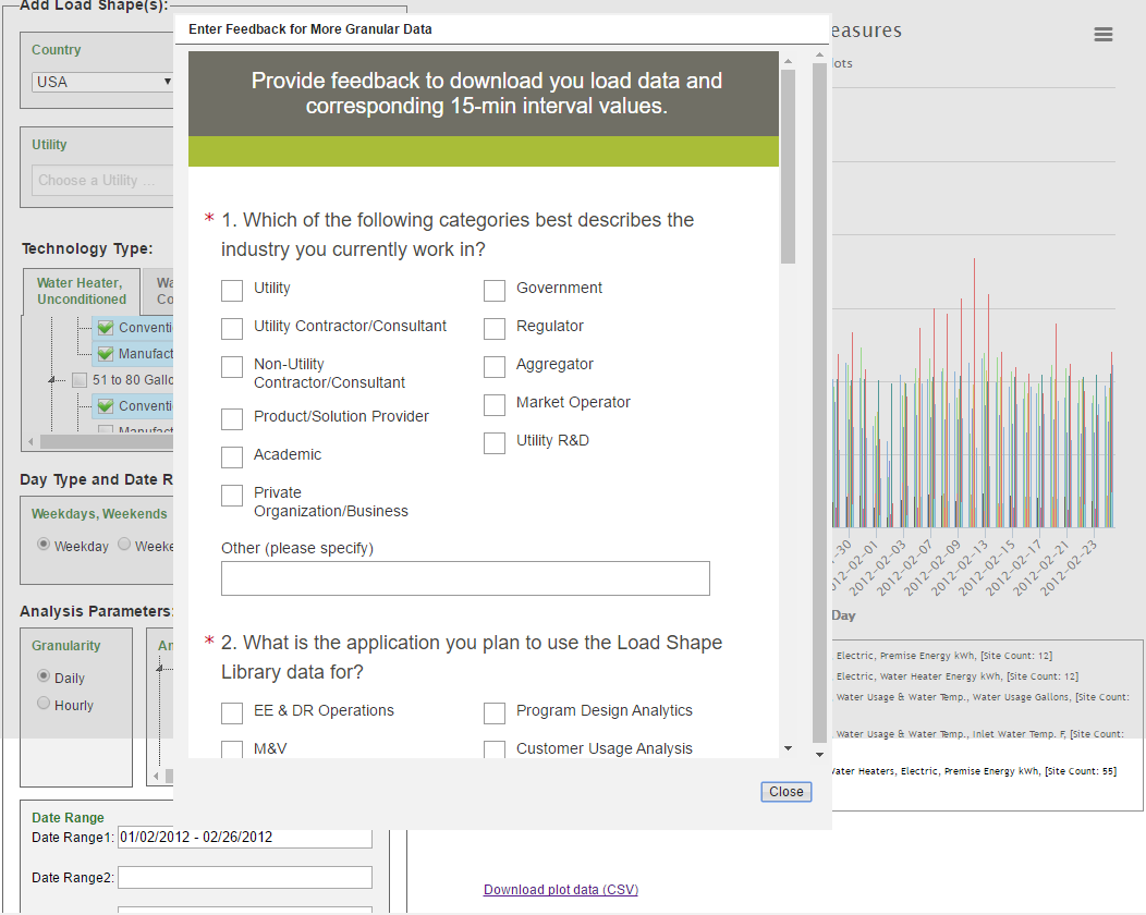
Step 9:
Alternatively, the user can select hourly granularity and plot load shapes as shown in Figure 3-12. If the user likes the plot, the data has the option of downloading the data for the plot and also the 15 minute time interval data for the same parameters. This can be achieved by filling out a simple survey on the page.
Figure 3-12
Technology Measures Download Data Plot
Technology Measures Download Data Plot
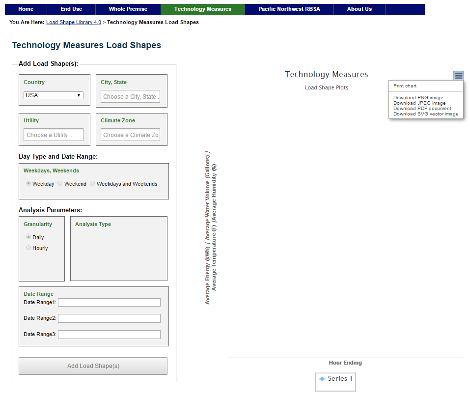
Step 10:
The user can print the plot or download the plot as an image in PNG or JPEG formats or as a PDF document or as a SVG vector image.
Figure 3-13
Technology Measures Print or Download Data Plot
Technology Measures Print or Download Data Plot
References
1. Curtis. A., AMI + MDMS: A Data Storage Conundrum, SCANA Energy, AEIC Load Research Workshop, Orlando, Florida, March 20 – 23, 2011↩
Open All
Close All
-
+
How do I access the Pacific Northwest RBSA Library?
The RBSA is a study sponsored by the Northwest Energy Efficiency Alliance (NEEA) in the Pacific Northwest region. The primary objective of the RBSA was to develop an inventory and profile of existing residential building stock in the Northwest based on field data from a representative, random sample of existing homes. The RBSA establishes the 2011 regional baseline for housing stock for three categories of residences: single-family homes, manufactured homes, and multifamily homes. The dataset used in the Load shape Library comprises of the following 1
- 103 single-family residential premises with end-use metered data
- The data ranges from April 2012- March 2013
- Data includes premises with electric and gas end-uses
EPRI used the dataset and the data contained within RBSA public database. No changes, or modifications or validations were conducted on the data except for the exclusion of gas end uses.
RBSA Load Shapes
Accessing the load data is similar to the steps outlined previously.
The user chooses the desired City or Utility or Climate Zone and Fuel Type at Premise for which load data is desired. The Fuel Type selection provides the choice to select all sites or sites with only electric as the fuel type at the premise or electric and gas as the fuel type at the premise.
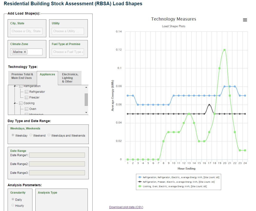
Under the technology type, the user then selects the end use or the end use category for which load shapes are desired. The user then selects the day type and the date range. The user selects the granularity of load shape and the desired analysis type parameter. The user clicks "Add Load Shapes" to plot the load shapes.
Figure Figure 3-14 shows the RBSA load shape page and the selections available for the user to access, visualize and download the desired end use data.
Figure 3-14
RBSA Plot
RBSA Plot
References
1. RBSA Single-Family Public Data Files https://neea.org/data/residential-building-stock-assessment ↩
For Support Contact:
|
Krish Gomatom (EPRI) |
Chris Holmes (EPRI) |
Paul Palathingal (Contract) |
OR
EPRI Customer Assistance Center
Phone: (800).313.3774
askepri@epri.com